Overview

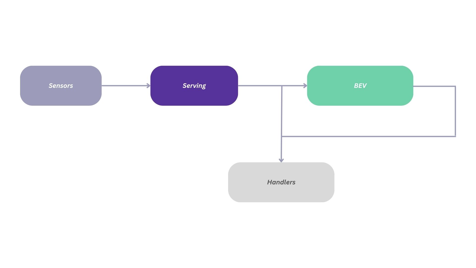
Here is an overview of the main components and concepts you need to know about Aloserving:

Pipeline: This is the main script you will use with Aloserving. It is meant to build a pipeline from the sensors all the way to the final application outputs.
Sensors: Sensors represent physical or virtual devices providing data about the environment. They provide a common interface for updating and retrieving data, either from actual live sensors, or from recorded data.
Serving Models: These are modules that encapsulate the logic for loading and executing machine learning models from Aloception. This is the so called baseline setup in your aloserving_configuration.yaml file.
BEV (Bird’s Eye View): This class is used to aggregate models predictions into a local map around the robot. BEV’s outputs can be used for motion planning and obstacle avoidance.

Pipeline

The Aloserving pipeline is a sequence of operations that are executed to process data from sensors all the way to the handlers. It can be configured and run using command line arguments or a YAML configuration file. The pipeline executes the following steps:

Read data from sensors
Run the serving models
Compute the outputs in the BEV
Publish the outputs on the protocol of your choice using handlers

To run the pipeline, you can use the pipeline_from_args.py script for command line arguments or the pipeline_from_yaml.py script for a YAML configuration file.

Note that the section Run your application is full of examples on how to run and configure your pipeline.

Sensors

In the context of the Aloserving library, a sensor is module class that represents a physical or virtual sensor. This could be a camera, a set of cameras or any other device that provides data about the environment.

Based on the sensor(s) you want to use, you should care about:

Calibration: Calibrating the camera intrinsics is very important to have accurate projection of the predicted depth in the 3D world.
High frequency: We recommend that your sensors streams close to 30 FPS so that Aloserving can run with as little latency as possible between multiple frames.
Synchronization: Because Aloception is running epipolar optimization internally, having synchronized frames is very important. This might be a particular concern when streaming your camera frames through ROS.
Recording: Being able to record datasets is important to replay particular scenarios or to improve the overall system performance over time. Aloserving provides you with several tools including a recording tool.

Serving

Serving models are modules that encapsulate the logic for loading and executing machine learning models. They are designed to provide a common interface for different types of models, making it easier to use them in a variety of contexts.

The main serving model that you will most likely use is the BEVServing model. It provides core information on the scene, including laserscan, obstacles, and explicitly modeled free space.

BEV (Bird’s Eye View)

The BEV class is used to aggregate the serving outputs into a local map around the robot that can be used for motion planning and obstacle avoidance. It provides methods for projecting data onto the map and committing new observations.

In bird’s-eye view mode, the height of the camera and its roll and pitch rotations are used to project information from the camera to the ground. Then in the BEV, only the translations on X and Z and the rotation on Y remain relevant.

Coordinate system

The coordinate systems used throughout the documentation and Aloserving follow the convention for a camera coordinate system, with y the vertical axis pointing down, z pointing forward and x to the right.

Camera coordinate system

The camera coordinate system is a 3D Cartesian coordinate system that is centered at the camera’s optical center (often termed the principal point). The axes are defined as:

X-axis: Horizontally across the image, perpendicular to the optical axis and typically oriented to the right when looking from behind the camera.
Y-axis: Vertically along the image, perpendicular to the optical axis, and typically oriented downward.
Z-axis (optical axis): Extending outward from the camera lens, oriented along the direction the camera is pointing. Positive values of Z move out from the camera into the scene.

BEV coordinate system

The BEV coordinate system is 2D. To remain consistent with the camera coordinate system we use X and Z to express the coordinates of a point in the 2D plane. It ensures an easy continuity from camera space to BEV space when the camera has no roll or pitch, or when considering the projection to the ground of the camera’s X and Z axis. To work with the BEV we thus use two representations of point coordinates:

When considering a point in the continuous space, we express its coordinates in meters with:

The X-axis colinear with the camera’s X-axis projected to the ground.
The Z-axis is colinear with the camera’s Z-axis projected to the ground.

When considering a pixel on a grid representation of the BEV (such as Occupancy or SemanticMap ), we use the convention for matrix coordinates where the first coordinate is written z and the second is written x. This gives the best continuity with previous notations, except that the matrix z coordinate is pointing downwards while the Z-axis from the metric representation points upwards on the BEV.

In practice, conversions to and from BEV coordinates require two parameters that define the geometry of the BEV grid:

px2m: the resolution of the grid, i.e. the meter size of a grid cell.
top_left_X and top_left_Z: the position of the top left corner of the map in meters, expressed in the coordinate system attached to the BEV grid.

To transform cell coordinates (x, z) in the occupancy matrix to world coordinates in meters (X, Z) with respect to the spatial frame attached to the occupancy grid:

X = top_left_X + x*px2m
Z = top_left_Z - z*px2m

And the other way around:

x = (X - top_left_X) / px2m
z = -(Z - top_left_Z) / px2m